Resilient supply chain planning & anomaly detection
When done properly, supply chain planning anomaly detection happens quickly and provides rapid (re-)planning across a value-stream. Balancing demand, inventory and supply, planning provides much greater flexibility and takes the variability of both demand and supply into consideration. It can replace physical buffers by rapid analysis of the as-is situation and prescriptive decision-making.
The cultural change is in realizing that the top plans of the past—both demand and supply—are history. The supply plan provides a range of demand satisfaction.
Unknown uncertainty toward known variability
As described in my previous blog, the smart parameter capability of Axon enables the parameter and value stream analysis to establish the demonstrated performance base line and to initiate performance improvement programs when the demonstrated performance is not in line with the desired performance.
Supply chain planning anomaly detection
Equally important is the tracking of these parameters through constant analysis to detect anomalies in expected values (mean, mode, median, etc.) and variability. An anomaly can be defined as a significant change in the expected value or variability. The moment an anomaly is detected, both the business process improvement and the planning team can be notified. Of course, the anomaly may have been triggered by a business improvement program, meaning we are moving from the demonstrated performance closer to the desired performance.
→ The key point is that the anomaly detection should trigger a change to the smart parameter value used in the legacy planning solution.
Types of anomalies
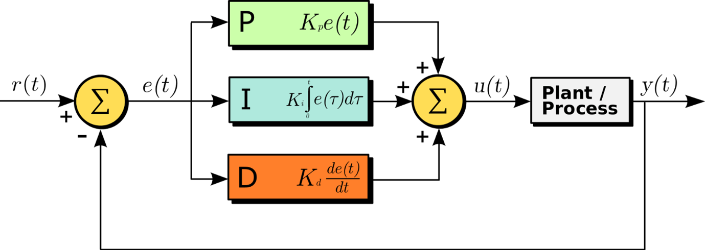
At the risk of asking you to dig deep into your knowledge of control theory, the classic PID practice is to capture three types of anomalies or errors:
- Offset (P)
- Persistent (I)
- Trend (D)

Offset anomaly
We are very used to the offset error from dashboards. The offset determines how far we are from the desired value and categorizes whether the difference is within or outside tolerance. Consequently, if the offset is outside the tolerance, it is considered as an offset anomaly. For instance, target revenue for the month of January 2021 was €20 million, our actual revenue was €15 million and so our “error” is -€5 million. This comes out to -25% of our target. If we set control limits of ±5%, this is an anomaly.
→ While the offset anomaly is used very frequently, I am of the opinion that it is the least useful because it is only triggered when there is a problem.
Persistent anomaly
The persistent anomaly is “death by a thousand cuts.” In other words, it is categorized as small enough errors that they do not trigger the offset anomaly detection but are consistently above or below the target. To expand on the revenue example above, let’s say that there has been a 1% (approximately) shortfall of revenue for the last 12 months. An anomaly would not have been triggered in any particular month because the offset control limits were never exceeded.
However, over a year, this would result in a 12% shortfall of revenue resulting in an undesirable situation.
→ Dashboards sometimes show persistent error, particularly for KPIs such as revenue, as cumulative attainment.
Trend anomaly
The trend anomaly captures a consistent change in the demonstrated performance metric. Again, the difference between demonstrated and desired performance in any period may not be enough to trigger the offset anomaly, but the error is changing in a consistent manner. For example, your revenue may have been +1% off target four months ago, +0.5% three months ago, 0% three months ago, -0.5% one month ago and -1% this month.
→ If this trend continues, in eight months, we will trigger the offset anomaly detection. As a result, it would be much better to take corrective action now to prevent the offset anomaly in eight months.
Mean and variability
What often gets missed in anomaly detection is that, not only should we be tracking demonstrated performance against the desired performance, but we should also be tracking the variability.

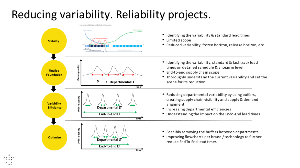
As shown in the diagram above, the first objective of an Axon customer is to reduce the variability of their lead time and then to reduce the overall lead time. This approach is very consistent with widely used Lean principles.
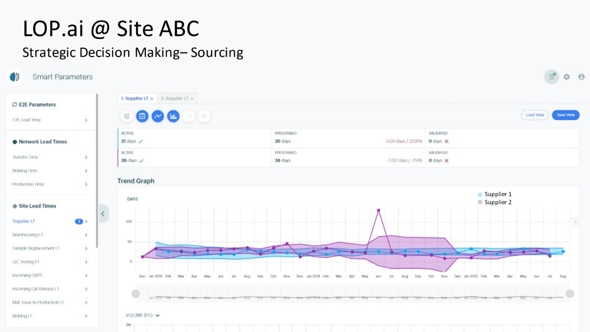
It becomes just as important to perform anomaly detection on the variability. In the diagram below, we can see the lead time performance of two suppliers of the same commodity to the same site:

There is little difference in the expected value/mean of the lead times from either supplier. However, there is an increase in variability of the lead time in the May to November 2019 period for Supplier 2. On the other hand, we see much reduced variability in the December 2019 to July 2020 period, which is very likely the result of a performance improvement program.
Summary
Axon not only provides areas of improvement in performance, but also provides smart parameters that can be fed to legacy planning systems. Additionally, it tracks changes in demonstrated performance, ultimately using them to alert on parameters that require immediate action and those that will result in poor performance at a later date if not addressed soon.
While Black Swan events, such as Covid-19, create a lot of disruption in supply chains, it is the daily changes in demonstrated performance that cause the greatest value loss in our supply chains.
As I wrote before, much has been written about resilient supply chains, particularly by Gartner, and by many of the management consulting companies. Here are a few examples:
- Gartner: 6 Strategies for a More Resilient Supply Chain
- McKinsey: Building Supply Chain Resilience
- BCG: Designing Resilience into Global Supply Chains
- Yossi Sheffi in HBR: Building a Resilient Supply Chain
- EY: How to Build Resilient Supply Chains in Times of Crisis


